Prior distributions in PEtab

This notebook gives a brief overview of the prior distributions in PEtab and how they are represented in the PEtab library.

Prior distributions are used to specify the prior knowledge about the parameters. Parameter priors are specified in the parameter table. A prior is defined by its type and its parameters. Each prior type has a specific set of parameters. For example, the normal distribution has two parameters: the mean and the standard deviation.

There are two types of priors in PEtab - objective priors and initialization priors:

• Objective priors are used to specify the prior knowledge about the parameters that are to be estimated. They will enter the objective function of the optimization problem. They are specified in the objectivePriorType and objectivePriorParameters columns of the parameter table.

• Initialization priors can be used as a hint for the optimization algorithm. They will not enter the objective function. They are specified in the initializationPriorType and initializationPriorParameters columns of the parameter table.

import matplotlib.pyplot as plt
import numpy as np
import seaborn as sns

from petab.v1.C import *
from petab.v1.parameters import unscale
from petab.v1.priors import Prior

sns.set_style(None)


def plot(prior: Prior):
    """Visualize a distribution."""
    fig, (ax1, ax2) = plt.subplots(1, 2, figsize=(12, 4))
    sample = prior.sample(20_000, x_scaled=True)

    fig.suptitle(str(prior))

    plot_single(prior, ax=ax1, sample=sample, scaled=False)
    plot_single(prior, ax=ax2, sample=sample, scaled=True)
    plt.tight_layout()
    plt.show()


def plot_single(
    prior: Prior, scaled: bool = False, ax=None, sample: np.array = None
):
    fig = None
    if ax is None:
        fig, ax = plt.subplots()

    if sample is None:
        sample = prior.sample(20_000)

    # assuming scaled sample
    if not scaled:
        sample = unscale(sample, prior.transformation)
        bounds = prior.bounds
    else:
        bounds = (
            (prior.lb_scaled, prior.ub_scaled)
            if prior.bounds is not None
            else None
        )

    # plot pdf
    xmin = min(
        sample.min(), bounds[0] if prior.bounds is not None else sample.min()
    )
    xmax = max(
        sample.max(), bounds[1] if prior.bounds is not None else sample.max()
    )
    padding = 0.1 * (xmax - xmin)
    xmin -= padding
    xmax += padding
    x = np.linspace(xmin, xmax, 500)
    y = prior.pdf(x, x_scaled=scaled, rescale=scaled)
    ax.plot(x, y, color="red", label="pdf")

    sns.histplot(sample, stat="density", ax=ax, label="sample")

    # plot bounds
    if prior.bounds is not None:
        for bound in bounds:
            if bound is not None and np.isfinite(bound):
                ax.axvline(bound, color="black", linestyle="--", label="bound")

    if fig is not None:
        ax.set_title(str(prior))

    if scaled:
        ax.set_xlabel(
            f"Parameter value on parameter scale ({prior.transformation})"
        )
        ax.set_ylabel("Rescaled density")
    else:
        ax.set_xlabel("Parameter value")

    ax.grid(False)
    handles, labels = ax.get_legend_handles_labels()
    unique_labels = dict(zip(labels, handles, strict=False))
    ax.legend(unique_labels.values(), unique_labels.keys())

    if ax is None:
        plt.show()

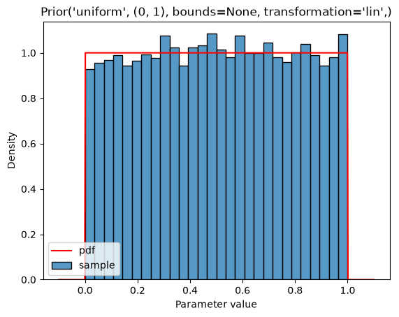
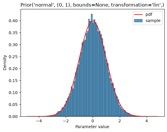
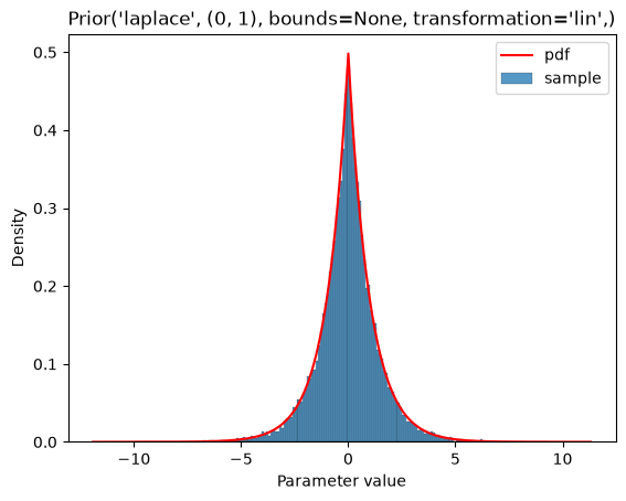
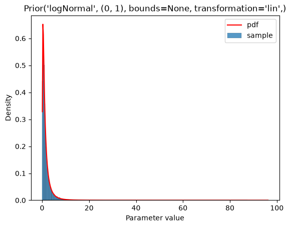
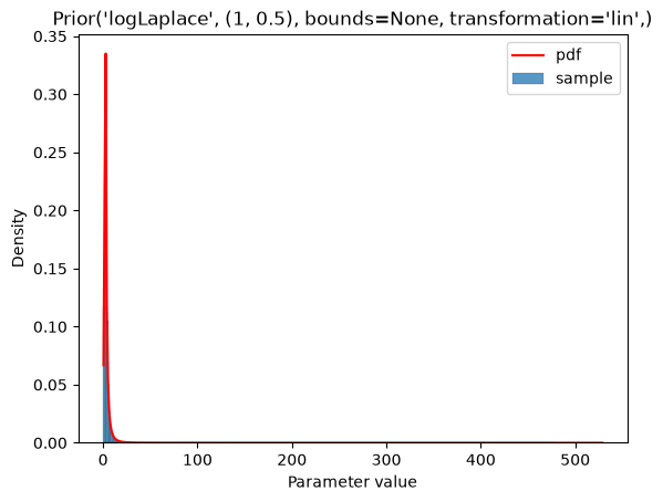
The basic distributions are the uniform, normal, Laplace, log-normal, and log-laplace distributions:

plot_single(Prior(UNIFORM, (0, 1)))
plot_single(Prior(NORMAL, (0, 1)))
plot_single(Prior(LAPLACE, (0, 1)))
plot_single(Prior(LOG_NORMAL, (0, 1)))
plot_single(Prior(LOG_LAPLACE, (1, 0.5)))

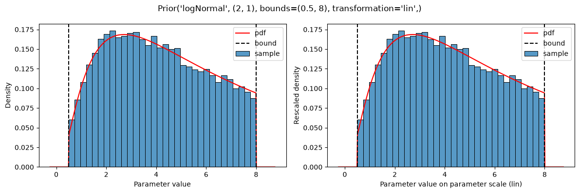
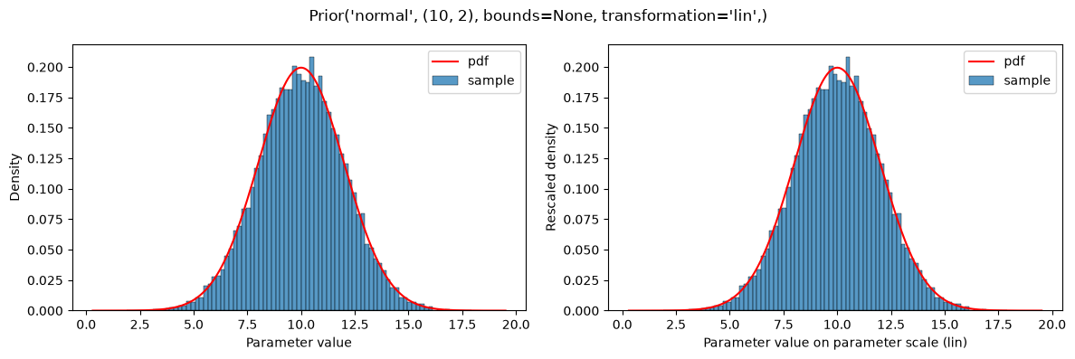
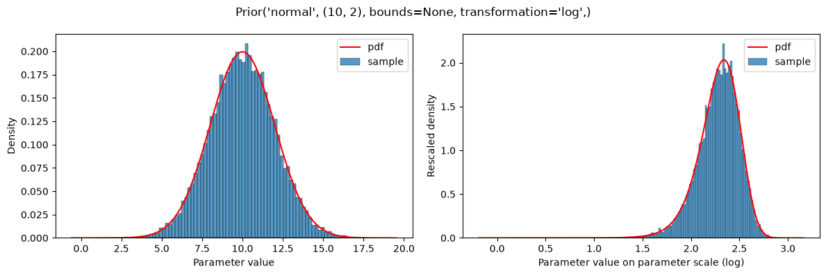
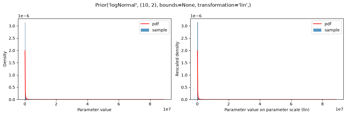
If a parameter scale is specified (parameterScale=lin|log|log10), the distribution parameters are used as is without applying the parameterScale to them. The exception are the parameterScale*-type distributions, as explained below. In the context of PEtab prior distributions, parameterScale will only be used for the start point sampling for optimization, where the sample will be transformed accordingly. This is demonstrated below. The left plot always shows the prior distribution for unscaled parameter values, and the right plot shows the prior distribution for scaled parameter values. Note that in the objective function, the prior is always on the unscaled parameters.

plot(Prior(NORMAL, (10, 2), transformation=LIN))
plot(Prior(NORMAL, (10, 2), transformation=LOG))

# Note that the log-normal distribution is different
#  from a log-transformed normal distribution:
plot(Prior(LOG_NORMAL, (10, 2), transformation=LIN))

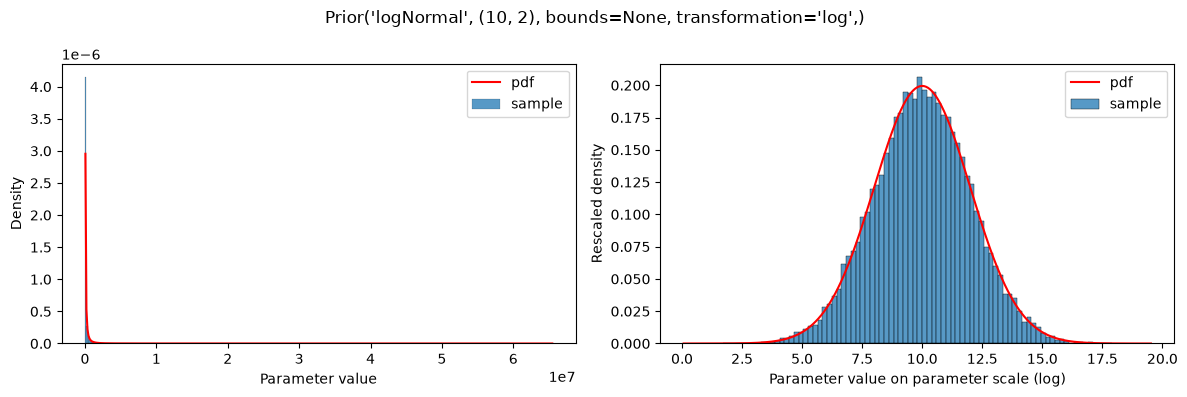
On the log-transformed parameter scale, Log* and parameterScale* distributions are equivalent:

plot(Prior(LOG_NORMAL, (10, 2), transformation=LOG))
plot(Prior(PARAMETER_SCALE_NORMAL, (10, 2)))

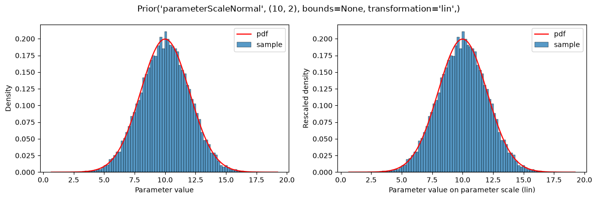
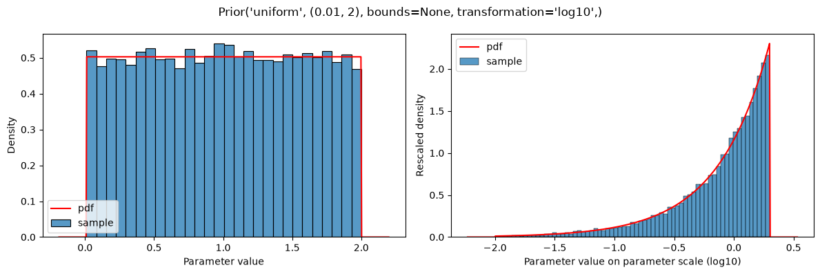
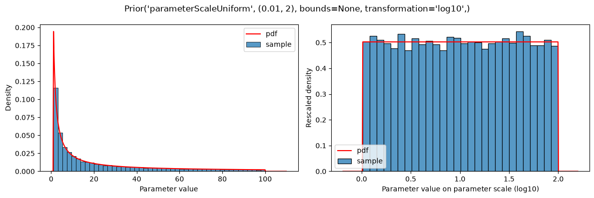
Prior distributions can also be defined on the scaled parameters (i.e., transformed according to parameterScale) by using the types parameterScaleUniform, parameterScaleNormal or parameterScaleLaplace. In these cases, the distribution parameters are interpreted on the transformed parameter scale (but not the parameter bounds, see below). This implies, that for parameterScale=lin, there is no difference between parameterScaleUniform and uniform.

# different, because transformation!=LIN
plot(Prior(UNIFORM, (0.01, 2), transformation=LOG10))
plot(Prior(PARAMETER_SCALE_UNIFORM, (0.01, 2), transformation=LOG10))

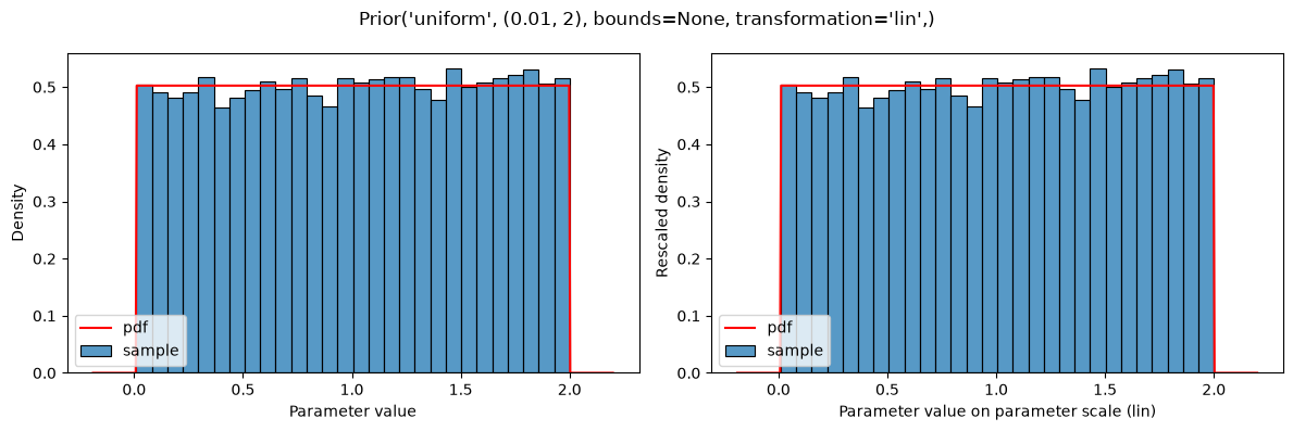
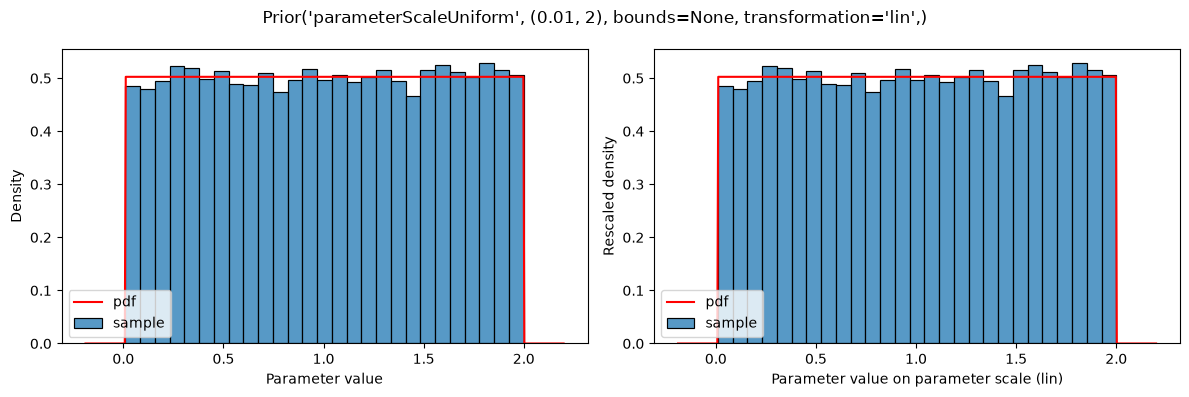
# same, because transformation=LIN
plot(Prior(UNIFORM, (0.01, 2), transformation=LIN))
plot(Prior(PARAMETER_SCALE_UNIFORM, (0.01, 2), transformation=LIN))

The given distributions are truncated at the bounds defined in the parameter table:

plot(Prior(NORMAL, (0, 1), bounds=(-2, 2)))
plot(Prior(UNIFORM, (0, 1), bounds=(0.1, 0.9)))
plot(Prior(UNIFORM, (1e-8, 1), bounds=(0.1, 0.9), transformation=LOG10))
plot(Prior(LAPLACE, (0, 1), bounds=(-0.5, 0.5)))
plot(
    Prior(
        PARAMETER_SCALE_UNIFORM,
        (-3, 1),
        bounds=(1e-2, 1),
        transformation=LOG10,
    )
)

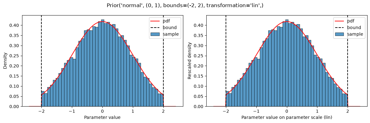
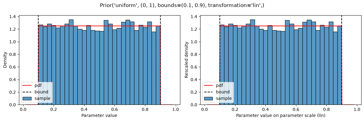
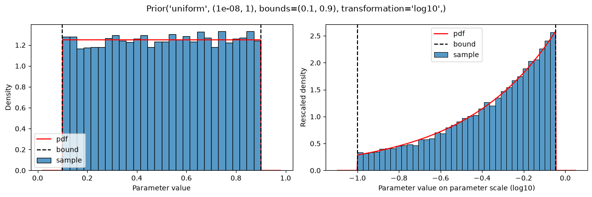
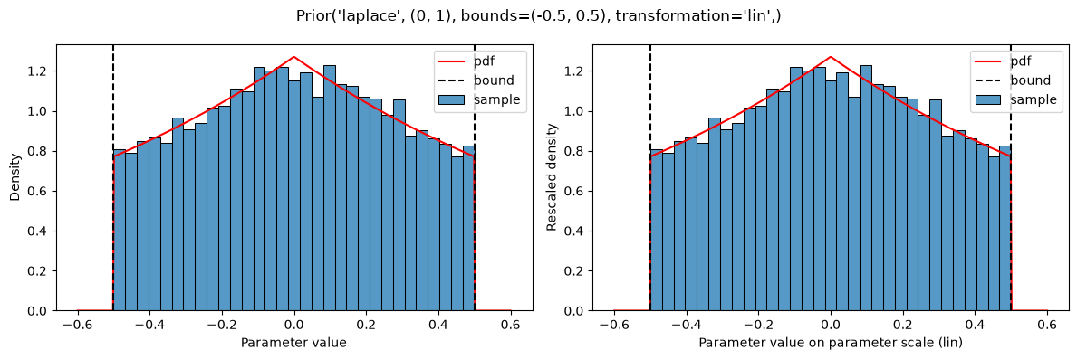
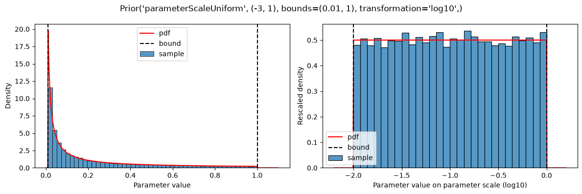
This results in a constant shift in the probability density, compared to the non-truncated version (https://en.wikipedia.org/wiki/Truncated_distribution), such that the probability density still sums to 1.

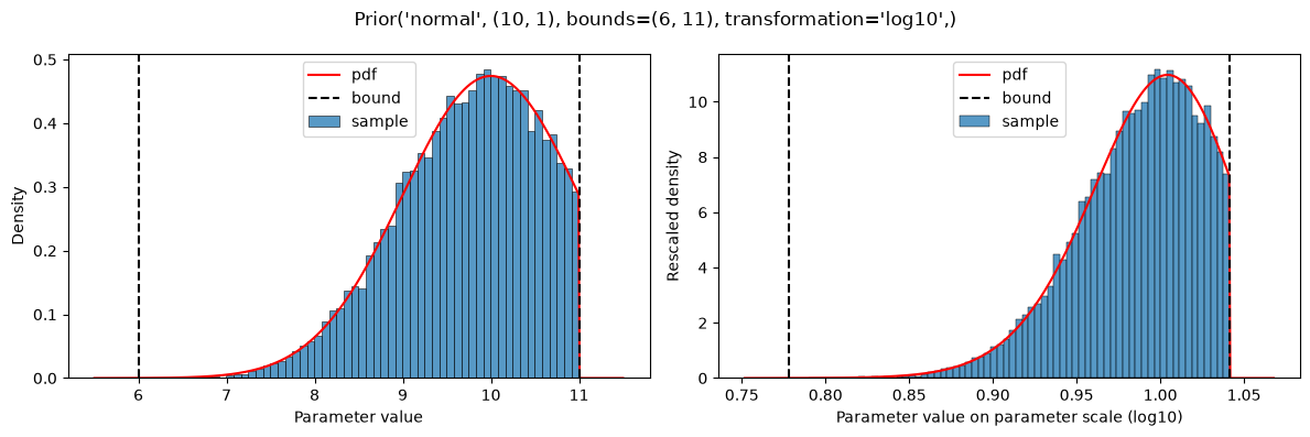
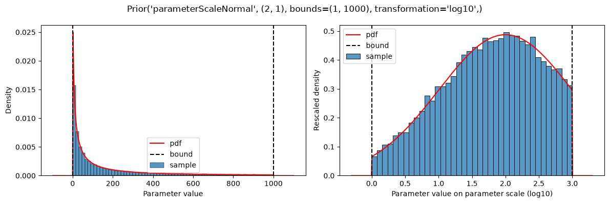
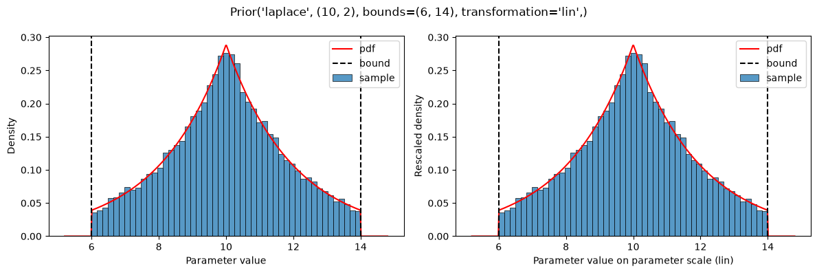
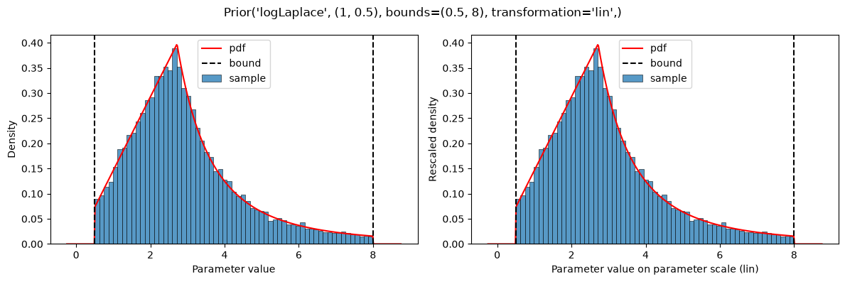
Further distribution examples:

plot(Prior(NORMAL, (10, 1), bounds=(6, 11), transformation="log10"))
plot(
    Prior(
        PARAMETER_SCALE_NORMAL,
        (2, 1),
        bounds=(10**0, 10**3),
        transformation="log10",
    )
)
plot(Prior(LAPLACE, (10, 2), bounds=(6, 14)))
plot(Prior(LOG_LAPLACE, (1, 0.5), bounds=(0.5, 8)))
plot(Prior(LOG_NORMAL, (2, 1), bounds=(0.5, 8)))