PEtab – a data format for specifying parameter estimation problems in systems biology¶

PEtab is a data format for specifying parameter estimation problems in systems biology. This repository provides extensive documentation and a Python library for easy access and validation of PEtab files.

About PEtab¶

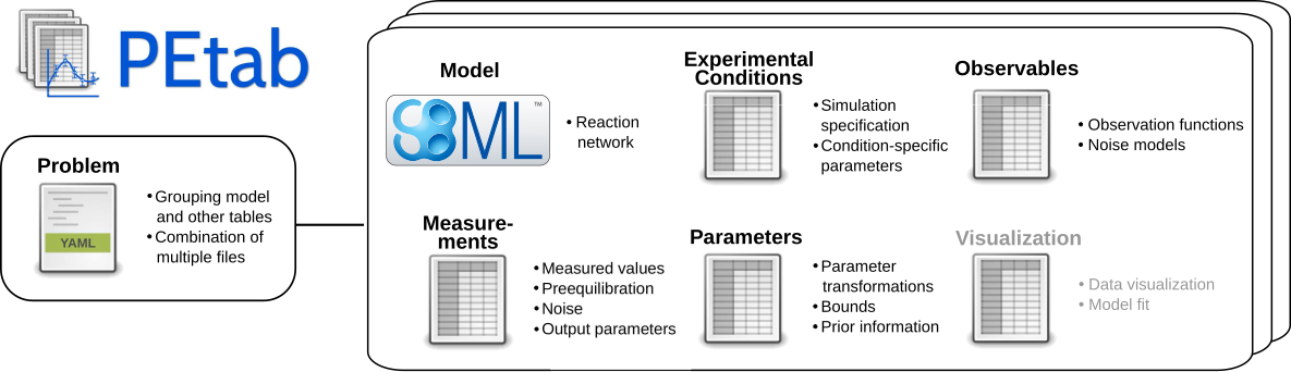
PEtab is built around SBML and based on tab-separated values (TSV) files. It is meant as a standardized way to provide information for parameter estimation, which is out of the current scope of SBML. This includes for example:

Specifying and linking measurements to models
- Defining model outputs
- Specifying noise models
Specifying parameter bounds for optimization
Specifying multiple simulation condition with potentially shared parameters

Documentation¶

Documentation of the PEtab data format and Python library is available at https://petab.readthedocs.io/en/latest/.

Examples¶

A wide range of PEtab examples can be found in the systems biology parameter estimation benchmark problem collection.

PEtab support in systems biology tools¶

Where PEtab is supported (in alphabetical order):

If your project or tool is using PEtab, and you would like to have it listed here, please let us know.

PEtab features supported in different tools¶

The following list provides an overview of supported PEtab features in different tools, based on passed test cases of the PEtab test suite:

ID	Test	AMICI `>=0.10.20`	Copasi	D2D	dMod	MEIGO	parPE `develop`	pyABC `>=0.10.1`	pyPESTO `>=0.0.11`
1	Basic simulation	+++	+–	+++	+++	+++	–+	+++	+++
2	Multiple simulation conditions	+++	+–	+++	+++	+++	–+	+++	+++
3	Numeric observable parameter overrides in measurement table	+++	+–	+++	+++	+++	–+	+++	+++
4	Parametric observable parameter overrides in measurement table	+++	+–	+++	+++	+++	–+	+++	+++
5	Parametric overrides in condition table	+++	+–	+++	+++	+++	–+	+++	+++
6	Time-point specific overrides in the measurement table	—	—	+++	+++	+++	—	—	—
7	Observable transformations to log10 scale	+-+	+–	+++	++-	+++	–+	+-+	+-+
8	Replicate measurements	+++	+–	+++	+++	+++	–+	+++	+++
9	Pre-equilibration	+++	+–	+++	+++	+++	–+	+++	+++
10	Partial pre-equilibration	+++	—	+++	+++	+++	–+	+++	+++
11	Numeric initial concentration in condition table	+++	+–	+++	+++	+++	–+	+++	+++
12	Numeric initial compartment sizes in condition table	—	+–	+++	+++	+++	—	—	—
13	Parametric initial concentrations in condition table	+++	+–	+++	+++	+++	–+	+++	+++
14	Numeric noise parameter overrides in measurement table	+++	+–	+++	+++	+++	–+	+++	+++
15	Parametric noise parameter overrides in measurement table	+++	+–	+++	+++	+++	–+	+++	+++
16	Observable transformations to log scale	+-+	+–	+++	++-	+++	–+	+-+	+-+

Legend:

First character indicates whether computing simulated data is supported and simulations are correct (+) or not (-).
Second character indicates whether computing chi2 values of residuals are supported and correct (+) or not (-).
Third character indicates whether computing likelihoods is supported and correct (+) or not (-).

Using PEtab¶

If you would like to use PEtab yourself, please have a look at doc/documentation_data_format.rst or at the example models provided in the benchmark collection.

To convert your existing parameter estimation problem to the PEtab format, you will have to:

Specify your model in SBML.
Create a condition table.
Create a table of observables.
Create a table of measurements.
Create a parameter table.

If you are using Python, some handy functions of the PEtab library can help you with that. This include also a PEtab validator called petablint which you can use to check if your files adhere to the PEtab standard. If you have further questions regarding PEtab, feel free to post an issue at our github repository.

PEtab Python library¶

PEtab comes with a Python package for creating, checking, visualizing and working with PEtab files. This library is available on pypi and the easiest way to install it is running

It will require Python>=3.6 to run.

Development versions of the PEtab library can be installed using

(replace develop by the branch or commit you would like to install).

When setting up a new parameter estimation problem, the most useful tools will be:

The PEtab validator, which is now automatically installed using Python entrypoints to be available as a shell command from anywhere called petablint
petab.create_parameter_df to create the parameter table, once you have set up the model, condition table, observable table and measurement table
petab.create_combine_archive to create a COMBINE Archive from PEtab files

Library examples¶

Examples for PEtab Python library usage:

Getting help¶

If you have any question or problems with PEtab, feel free to post them at our GitHub issue tracker.

Contributing to PEtab¶

Contributions and feedback to PEtab are very welcome, see our contribution guide.

PEtab data format specification¶

Format version: 1

This document explains the PEtab data format.

Purpose¶

Providing a standardized way for specifying parameter estimation problems in systems biology, especially for the case of Ordinary Differential Equation (ODE) models.

Overview¶

The PEtab data format specifies a parameter estimation problem using a number of text-based files (Systems Biology Markup Language (SBML) and Tab-Separated Values (TSV)), i.e.

An SBML model [SBML]
A measurement file to fit the model to [TSV]
A condition file specifying model inputs and condition-specific parameters [TSV]
An observable file specifying the observation model [TSV]
A parameter file specifying optimization parameters and related information [TSV]
(optional) A simulation file, which has the same format as the measurement file, but contains model simulations [TSV]
(optional) A visualization file, which contains specifications how the data and/or simulations should be plotted by the visualization routines [TSV]

The following sections will describe the minimum requirements of those components in the core standard, which should provide all information for defining the parameter estimation problem.

Extensions of this format (e.g. additional columns in the measurement table) are possible and intended. However, while those columns may provide extra information for example for plotting, downstream analysis, or for more efficient parameter estimation, they should not affect the optimization problem as such.

General remarks

All model entities, column names and row names are case-sensitive
All identifiers must consist only of upper and lower case letters, digits and underscores, and must not start with a digit.
Fields in “[]” are optional and may be left empty.

SBML model definition¶

The model must be specified as valid SBML. There are no further restrictions.

Condition table¶

The condition table specifies parameters, or initial values of species and compartments for specific simulation conditions (generally corresponding to different experimental conditions).

This is specified as a tab-separated value file in the following way:

conditionId	[conditionName]	parameterOrSpeciesOrCompartmentId1	…	parameterOrSpeciesOrCompartmentId${n}
STRING	[STRING]	NUMERIC\|STRING	…	NUMERIC\|STRING
e.g.
conditionId1	[conditionName1]	0.42	…	parameterId
conditionId2	…	…	…	…
…	…	…	…

Row- and column-ordering are arbitrary, although specifying conditionId first may improve human readability.

Additional columns are not allowed.

Detailed field description¶

conditionId [STRING, NOT NULL]

Unique identifier for the simulation/experimental condition, to be referenced by the measurement table described below.
conditionName [STRING, OPTIONAL]

Condition names are arbitrary strings to describe the given condition. They may be used for reporting or visualization.
${parameterOrSpeciesOrCompartmentId1}

Further columns may be global parameter IDs, IDs of species or compartments as defined in the SBML model. Only one column is allowed per ID. Values for these condition parameters may be provided either as numeric values, or as IDs defined in the SBML model, the parameter table or both.
- ${parameterId}
  
  The values will override any parameter values specified in the model.
- ${speciesId}
  
  If a species ID is provided, it is interpreted as the initial concentration/amount of that species and will override the initial concentration/amount given in the SBML model or given by a preequilibration condition. If NaN is provided for a condition, the result of the preequilibration (or initial concentration/amount from the SBML model, if no preequilibration is defined) is used.
- ${compartmentId}
  
  If a compartment ID is provided, it is interpreted as the initial compartment size.

Measurement table¶

A tab-separated values files containing all measurements to be used for model training or validation.

Expected to have the following named columns in any (but preferably this) order:

observableId	[preequilibrationConditionId]	simulationConditionId	measurement	time
observableId	[conditionId]	conditionId	NUMERIC	NUMERIC\|inf
…	…	…	…	…

(wrapped for readability)

…	[observableParameters]	[noiseParameters]
…	[parameterId\|NUMERIC[;parameterId\|NUMERIC][…]]	[parameterId\|NUMERIC[;parameterId\|NUMERIC][…]]
…	…	…

Additional (non-standard) columns may be added. If the additional plotting functionality of PEtab should be used, such columns could be

…	[datasetId]	[replicateId]
…	[datasetId]	[replicateId]
…	…	…

where datasetId is a necessary column to use particular plotting functionality, and replicateId is optional, which can be used to group replicates and plot error bars.

Detailed field description¶

observableId [STRING, NOT NULL, REFERENCES(observables.observableID)]

Observable ID as defined in the observables table described below.
preequilibrationConditionId [STRING OR NULL, REFERENCES(conditionsTable.conditionID), OPTIONAL]

The conditionId to be used for preequilibration. E.g. for drug treatments, the model would be preequilibrated with the no-drug condition. Empty for no preequilibration.
simulationConditionId [STRING, NOT NULL, REFERENCES(conditionsTable.conditionID)]

conditionId as provided in the condition table, specifying the condition-specific parameters used for simulation.
measurement [NUMERIC, NOT NULL]

The measured value in the same units/scale as the model output.
time [NUMERIC OR STRING, NOT NULL]

Time point of the measurement in the time unit specified in the SBML model, numeric value or inf (lower-case) for steady-state measurements.
observableParameters [NUMERIC, STRING OR NULL, OPTIONAL]

This field allows overriding or introducing condition-specific versions of output parameters defined in the observation model. The model can define observables (see below) containing place-holder parameters which can be replaced by condition-specific dynamic or constant parameters. Placeholder parameters must be named observableParameter${n}_${observableId} with n ranging from 1 (not 0) to the number of placeholders for the given observable, without gaps. If the observable specified under observableId contains no placeholders, this field must be empty. If it contains n > 0 placeholders, this field must hold n semicolon-separated numeric values or parameter names. No trailing semicolon must be added.

Different lines for the same observableId may specify different parameters. This may be used to account for condition-specific or batch-specific parameters. This will translate into an extended optimization parameter vector.

All placeholders defined in the observation model must be overwritten here. If there are no placeholders used, this column may be omitted.
noiseParameters [NUMERIC, STRING OR NULL, OPTIONAL]

The measurement standard deviation or NaN if the corresponding sigma is a model parameter.

Numeric values or parameter names are allowed. Same rules apply as for observableParameters in the previous point.
datasetId [STRING, OPTIONAL]

The datasetId is used to group certain measurements to datasets. This is typically the case for data points which belong to the same observable, the same simulation and preequilibration condition, the same noise model, the same observable transformation and the same observable parameters. This grouping makes it possible to use the plotting routines which are provided in the PEtab repository.
replicateId [STRING, OPTIONAL]

The replicateId can be used to discern replicates with the same datasetId, which is helpful for plotting e.g. error bars.

Observables table¶

Parameter estimation requires linking experimental observations to the model of interest. Therefore, one needs to define observables (model outputs) and respective noise models, which represent the measurement process. Since parameter estimation is beyond the scope of SBML, there exists no standard way to specify observables (model outputs) and respective noise models. Therefore, in PEtab observables are specified in a separate table as described in the following. This allows for a clear separation of the observation model and the underlying dynamic model, which allows, in most cases, to reuse any existing SBML model without modifications.

The observable table has the following columns:

observableId	[observableName]	observableFormula
STRING	[STRING]	STRING
e.g.
relativeTotalProtein1	Relative abundance of Protein1	observableParameter1_relativeTotalProtein1 * (protein1 + phospho_protein1 )
…	…	…

(wrapped for readability)

…	[observableTransformation]	noiseFormula	[noiseDistribution]
…	[lin(default)\|log\|log10]	STRING\|NUMBER	[laplace\|normal]
…	e.g.
…	lin	noiseParameter1_relativeTotalProtein1	normal
…	…	…	…

Detailed field description¶

observableId [STRING]

Any identifier which would be a valid identifier in SBML. This is referenced by the observableId column in the measurement table. Must be different from any existing model entity or parameter introduced elsewhere.
[observableName] [STRING, OPTIONAL]

Name of the observable. Only used for output, not for identification.
observableFormula [STRING]

Observation function as plain text formula expression. May contain any symbol defined in the SBML model (including model time time) or parameter table. In the simplest case just an SBML species ID or an AssignmentRule target.

May introduce new parameters of the form observableParameter${n}_${observableId}, which are overridden by observableParameters in the measurement table (see description there).

observableTransformation [STRING, OPTIONAL]

Transformation of the observable and measurement for computing the objective function. Must be one of lin, log or log10. Defaults to lin. The measurements and model outputs are both assumed to be provided in linear space.

noiseFormula [NUMERIC|STRING]

Measurement noise can be specified as a numerical value which will default to a Gaussian noise model if not specified differently in noiseDistribution with standard deviation as provided here. In this case, the same standard deviation is assumed for all measurements for the given observable.

Alternatively, some formula expression can be provided to specify more complex noise models. A noise model which accounts for relative and absolute contributions could, e.g., be defined as:
```
noiseParameter1_observable_pErk + noiseParameter2_observable_pErk*pErk
```
with noiseParameter1_observable_pErk denoting the absolute and noiseParameter2_observable_pErk the relative contribution for the observable observable_pErk corresponding to species pErk. IDs of noise parameters that need to have different values for different measurements have the structure: noiseParameter${indexOfNoiseParameter}_${observableId} to facilitate automatic recognition. The specific values or parameters are assigned in the noiseParameters field of the measurement table (see above). Any parameters named noiseParameter${1..n}_${observableId} must be overwritten in the measurement table.

noiseDistribution [STRING: ‘normal’ or ‘laplace’, OPTIONAL]

Assumed noise distribution for the given measurement. Only normally or Laplace distributed noise is currently allowed (log-normal and log-Laplace are obtained by setting observableTransformation to log, similarly for log10). Defaults to normal. If normal, the specified noiseParameters will be interpreted as standard deviation (not variance). If Laplace ist specified, the specified noiseParameter will be interpreted as the scale, or diversity, parameter.

Noise distributions¶

For noiseDistribution, normal and laplace are supported. For observableTransformation, lin, log and log10 are supported. Denote by $y$ the simulation, $m$ the measurement, and $\sigma$ the standard deviation of a normal, or the scale parameter of a laplace model, as given via the noiseFormula field. Then we have the following effective noise distributions.

Normal distribution:

\[\pi(m|y,\sigma) = \frac{1}{\sqrt{2\pi}\sigma}\exp\left(-\frac{(m-y)^2}{2\sigma^2}\right)\]
Log-normal distribution (i.e. log(m) is normally distributed):

\[\pi(m|y,\sigma) = \frac{1}{\sqrt{2\pi}\sigma m}\exp\left(-\frac{(\log m - \log y)^2}{2\sigma^2}\right)\]
Log10-normal distribution (i.e. log10(m) is normally distributed):

\[\pi(m|y,\sigma) = \frac{1}{\sqrt{2\pi}\sigma m \log(10)}\exp\left(-\frac{(\log_{10} m - \log_{10} y)^2}{2\sigma^2}\right)\]
Laplace distribution:

\[\pi(m|y,\sigma) = \frac{1}{2\sigma}\exp\left(-\frac{|m-y|}{\sigma}\right)\]
Log-Laplace distribution (i.e. log(m) is Laplace distributed):

\[\pi(m|y,\sigma) = \frac{1}{2\sigma m}\exp\left(-\frac{|\log m - \log y|}{\sigma}\right)\]
Log10-Laplace distribution (i.e. log10(m) is Laplace distributed):

\[\pi(m|y,\sigma) = \frac{1}{2\sigma m \log(10)}\exp\left(-\frac{|\log_{10} m - \log_{10} y|}{\sigma}\right)\]

The distributions above are for a single data point. For a collection $D=\{m_i\}_i$ of data points and corresponding simulations $Y=\{y_i\}_i$ and noise parameters $\Sigma=\{\sigma_i\}_i$, the current specification assumes independence, i.e. the full distributions is

\[\pi(D|Y,\Sigma) = \prod_i\pi(m_i|y_i,\sigma_i)\]

Parameter table¶

A tab-separated value text file containing information on model parameters.

This table must include the following parameters:

Named parameter overrides introduced in the conditions table, unless defined in the SBML model
Named parameter overrides introduced in the measurement table

and must not include:

Placeholder parameters (see observableParameters and noiseParameters above)
Parameters included as column names in the condition table
Parameters that are AssignmentRule targets in the SBML model

it may include:

Any SBML model parameter that was not excluded above
Named parameter overrides introduced in the conditions table

One row per parameter with arbitrary order of rows and columns:

parameterId	[parameterName]	parameterScale	lowerBound	upperBound	nominalValue	estimate	…
STRING	[STRING]	log10\|lin\|log	NUMERIC	NUMERIC	NUMERIC	0\|1	…
…	…	…	…	…	…	…	…

(wrapped for readability)

…	[initializationPriorType]	[initializationPriorParameters]	[objectivePriorType]	[objectivePriorParameters]
…	see below	see below	see below	see below
…	…	…	…	…

Additional columns may be added.

Detailed field description¶

parameterId [STRING, NOT NULL]

The parameterId of the parameter described in this row. This has to match the ID of a parameter specified in the SBML model, a parameter introduced as override in the condition table, or a parameter occurring in the observableParameters or noiseParameters column of the measurement table (see above).
parameterName [STRING, OPTIONAL]

Parameter name to be used e.g. for plotting etc. Can be chosen freely. May or may not coincide with the SBML parameter name.
parameterScale [lin|log|log10]

Scale of the parameter to be used during parameter estimation.
lowerBound [NUMERIC]

Lower bound of the parameter used for optimization. Optional, if estimate==0. Must be provided in linear space, independent of parameterScale.
upperBound [NUMERIC]

Upper bound of the parameter used for optimization. Optional, if estimate==0. Must be provided in linear space, independent of parameterScale.
nominalValue [NUMERIC]

Some parameter value to be used if the parameter is not subject to estimation (see estimate below). Must be provided in linear space, independent of parameterScale. Optional, unless estimate==0.
estimate [BOOL 0|1]

1 or 0, depending on, if the parameter is estimated (1) or set to a fixed value(0) (see nominalValue).
initializationPriorType [STRING, OPTIONAL]

Prior types used for sampling of initial points for optimization. Sampled points are clipped to lie inside the parameter boundaries specified by lowerBound and upperBound. Defaults to parameterScaleUniform.

Possible prior types are:
- uniform: flat prior on linear parameters
- normal: Gaussian prior on linear parameters
- laplace: Laplace prior on linear parameters
- logNormal: exponentiated Gaussian prior on linear parameters
- logLaplace: exponentiated Laplace prior on linear parameters
- parameterScaleUniform (default): Flat prior on original parameter scale (equivalent to “no prior”)
- parameterScaleNormal: Gaussian prior on original parameter scale
- parameterScaleLaplace: Laplace prior on original parameter scale
initializationPriorParameters [STRING, OPTIONAL]

Prior parameters used for sampling of initial points for optimization, separated by a semicolon. Defaults to lowerBound;upperBound.

So far, only numeric values will be supported, no parameter names. Parameters for the different prior types are:
- uniform: lower bound; upper bound
- normal: mean; standard deviation (not variance)
- laplace: location; scale
- logNormal: parameters of corresp. normal distribution (see: normal)
- logLaplace: parameters of corresp. Laplace distribution (see: laplace)
- parameterScaleUniform: lower bound; upper bound
- parameterScaleNormal: mean; standard deviation (not variance)
- parameterScaleLaplace: location; scale
objectivePriorType [STRING, OPTIONAL]

Prior types used for the objective function during optimization or sampling. For possible values, see initializationPriorType.
objectivePriorParameters [STRING, OPTIONAL]

Prior parameters used for the objective function during optimization. For more detailed documentation, see initializationPriorParameters.

Visualization table¶

A tab-separated value file containing the specification of the visualization routines which come with the PEtab repository. Plots are in general collections of different datasets as specified using their datasetId (if provided) inside the measurement table.

Expected to have the following columns in any (but preferably this) order:

plotId	[plotName]	[plotTypeSimulation]	[plotTypeData]
STRING	[STRING]	[LinePlot(default)\|BarPlot\|ScatterPlot]	[MeanAndSD(default)\|MeanAndSEM\|replicate;provided]
…	…	…	…

(wrapped for readability)

…	[datasetId]	[xValues]	[xOffset]	[xLabel]	[xScale]
…	[datasetId]	[time(default)\|parameterOrStateId]	[NUMERIC]	[STRING]	[lin\|log\|log10\|order]
…	…	…	…	…	…

(wrapped for readability)

…	[yValues]	[yOffset]	[yLabel]	[yScale]	[legendEntry]
…	[observableId]	[NUMERIC]	[STRING]	[lin\|log\|log10]	[STRING]
…	…	…	…	…	…

Detailed field description¶

plotId [STRING, NOT NULL]

An ID which corresponds to a specific plot. All datasets with the same plotId will be plotted into the same axes object.
plotName [STRING, OPTIONAL]

A name for the specific plot.
plotTypeSimulation [STRING, OPTIONAL]

The type of the corresponding plot, can be LinePlot, BarPlot and ScatterPlot. Default is LinePlot.
plotTypeData [STRING, OPTIONAL]

The type how replicates should be handled, can be MeanAndSD, MeanAndSEM, replicate (for plotting all replicates separately), or provided (if numeric values for the noise level are provided in the measurement table). Default is MeanAndSD.
datasetId [STRING, NOT NULL, REFERENCES(measurementTable.datasetId), OPTIONAL]

The datasets which should be grouped into one plot.
xValues [STRING, OPTIONAL]

The independent variable, which will be plotted on the x-axis. Can be time (default, for time resolved data), or it can be parameterOrStateId for dose-response plots. The corresponding numeric values will be shown on the x-axis.
xOffset [NUMERIC, OPTIONAL]

Possible data-offsets for the independent variable (default is 0).
xLabel [STRING, OPTIONAL]

Label for the x-axis. Defaults to the entry in xValues.
xScale [STRING, OPTIONAL]

Scale of the independent variable, can be lin, log, log10 or order. The order value should be used if values of the independent variable are ordinal. This value can only be used in combination with LinePlot value for the plotTypeSimulation column. In this case, points on x axis will be placed equidistantly from each other. Default is lin.
yValues [observableId, REFERENCES(measurementTable.observableId), OPTIONAL]

The observable which should be plotted on the y-axis.
yOffset [NUMERIC, OPTIONAL]

Possible data-offsets for the observable (default is 0).
yLabel [STRING, OPTIONAL]

Label for the y-axis. Defaults to the entry in yValues.
yScale [STRING, OPTIONAL]

Scale of the observable, can be lin, log, or log10. Default is lin.
legendEntry [STRING, OPTIONAL]

The name that should be displayed for the corresponding dataset in the legend and which defaults to the value in datasetId.

Extensions¶

Additional columns, such as Color, etc. may be specified.

Examples¶

Examples of the visualization table can be found in the Benchmark model collection, for example in the Chen_MSB2009 model.

YAML file for grouping files¶

To link the SBML model, measurement table, condition table, etc. in an unambiguous way, we use a YAML file.

This file also allows specifying a PEtab version (as the format is not unlikely to change in the future).

Furthermore, this can be used to describe parameter estimation problems comprising multiple models (more details below).

The format is described in the schema ../petab/petab_schema.yaml, which allows for easy validation.

Parameter estimation problems combining multiple models¶

Parameter estimation problems can comprise multiple models. For now, PEtab allows to specify multiple SBML models with corresponding condition and measurement tables, and one joint parameter table. This means that the parameter namespace is global. Therefore, parameters with the same ID in different models will be considered identical.

API Reference¶

`petab`	PEtab global
`petab.composite_problem`	PEtab problems consisting of multiple models
`petab.core`	PEtab core functions (or functions that don’t fit anywhere else)
`petab.conditions`	Functions operating on the PEtab condition table
`petab.C`	This file contains constant definitions.
`petab.lint`	Integrity checks and tests for specific features used
`petab.measurements`	Functions operating on the PEtab measurement table
`petab.parameter_mapping`	Functions related to mapping parameter from model to parameter estimation problem
`petab.parameters`	Functions operating on the PEtab parameter table
`petab.problem`	PEtab Problem class
`petab.sampling`	Functions related to parameter sampling
`petab.sbml`	Functions for interacting with SBML models
`petab.yaml`	Code regarding the PEtab YAML config files
`petab.visualize.data_overview`	Functions for creating an overview report of a PEtab problem
`petab.visualize.helper_functions`	This file should contain the functions, which PEtab internally needs for plotting, but which are not meant to be used by non-developers and should hence not be directly visible/usable when using import petab.visualize.
`petab.visualize.plot_data_and_simulation`(…)	Main function for plotting data and simulations.
`petab.visualize.plotting_config`	Plotting config

PEtab changelog¶

0.1 series¶

0.1.10¶

Fixed deployment setup, no further changes.

0.1.9¶

Library:

Allow URL as filenames for YAML files and SBML models (Closes #187) (#459)
Allow model time in observable formulas (#445)
Make float parsing from CSV round-trip (#444)
Validator: Error message for missing IDs, with line numbers. (#467)
Validator: Detect duplicated observable IDs (#446)
Some documentation and CI fixes / updates
Visualization: Add option to save visualization specification (#457)
Visualization: Column XValue not mandatory anymore (#429)
Visualization: Add sorting of indices of dataframes for the correct sorting of x-values (#430)
Visualization: Default value for the column x_label in vis_spec (#431)

0.1.8¶

Library:

Use core.is_empty to check for empty values (#434)
Move tests to python 3.8 (#435)
Update to libcombine 0.2.6 (#437)
Make float parsing from CSV round-trip (#444)
Lint: Allow model time in observable formulas (#445)
Lint: Detect duplicated observable ids (#446)
Fix likelihood calculation with missing values (#451)

Documentation:

Move format documentation to restructuredtext format (#452)
Document all noise distributions and observable scales (#452)
Fix documentation for prior distribution (#449)

Visualization:

Make XValue column non-mandatory (#429)
Apply correct condition sorting (#430)
Apply correct default x label (#431)

0.1.7¶

Documentation:

Update coverage and links of supporting tools
Update explanatory figure

0.1.6¶

Library:

Fix handling of empty columns for residual calculation (#392)
Allow optional fixing of fixed parameters in parameter mapping (#399)
Fix function to flatten out time-point specific overrides (#404)
Add function to create a problem yaml file (#398)
Allow merging of multiple parameter files (#407)

Documentation:

In README, add to the overview table the coverage for the supporting tools, and links and usage examples (various commits)
Show REAMDE on readthedocs documentation front page (#400)
Correct description of observable and noise formulas (#401)
Update documentation on optional visualization values (#405, #419)

Visualization:

Fix sorting problem (#396)
More generously handle optional values (#405, #419)
Create dataset id also for simulation dataframe (#408)
Extend test suite for visualization (#418)

0.1.5¶

Library:

New create empty observable function (issue 386) (#387)
Deprecate petab.sbml.globalize_parameters (#381)
Fix computing log10 likelihood (#380)
Documentation update and typehints for visualization (#372)
Ordered result of petab.get_output_parameters
Fix missing argument to parameters.create_parameter_df

Documentation:

Add overview of supported PEtab feature in toolboxes
Add contribution guide
Fix optional values in documentation (#378)

0.1.4¶

Library:

Fixes / updates in functions for computing llh and chi2
Allow and require output parameters defined in observable table to be defined in parameter table
Fix merge_preeq_and_sim_pars_condition which incorrectly assumed lists instead of dicts
Update parameter mapping to deal with species and compartments in condition table
Removed petab.migrations.sbml_observables_to_table

For converting older PEtab files to observable table format, use one of the previous releases
Visualization:
- Fix various issues with get_data_to_plot
- Fixed various issues with expected presence of optional columns

0.1.3¶

File format:

Updated documentation
Observables table in YAML file now mandatory in schema (was implicitly mandatory before, as observable table was required already)

Library:

petablint:
- Fix: allow specifying observables file via CLI (Closes #302)
- Fix: nominalValue is optional unless estimated!=1 anywhere (Fixes #303)
- Fix: handle undefined observables more gracefully (Closes #300) (#351)
Parameter mapping:
- Fix / refactor parameter mapping (breaking change) (#344) (now performing parameter value and scale mapping together)
- check optional measurement cols in mapping (#350)
allow calculating llhs (#349), chi2 values (#348) and residuals (#345)
Visualization
- Basic Scatterplots & lot of bar plot fixes (#270)
- Fix incorrect length of bool bool_preequ when subsetting with ind_meas (Closes #322)
make libcombine optional (#338)

0.1.2¶

Library:

Extensions and fixes for the visualization functions (#255, #262)
Allow to extract fixed|free and scaled|non-scaled parameters (#256, #268, #273)
Various fixes (esp. #264)
Add function to get observable ids (#269)
Improve documentation (esp. #289)
Set default column for simulation results to ‘simulation’
Add support for COMBINE archives (#271)
Fix sbml observables to table
Improve prior and dataframe tests (#285, #286, #297)
Add function to get parameter table with all default values (#288)
Move tests to github actions (#281)
Check for valid identifiers
Fix handling of empty values in dataframes
Allow to get numeric values in parameter mappings in scaled form (#308)

0.1.1¶

Library:

Fix parameter mapping: include output parameters not present in SBML model
Fix missing petab/petab_schema.yaml in source distribution
Let get_placeholders return an (ordered) list of placeholders
Deprecate petab.problem.from_folder and related functions (obsolete after introducing more flexible YAML files for grouping tables and models)

0.1.0¶

Data format:

Introduce observables table instead of SBML assignment rules for defining observation model (#244) (moves observableTransformation and noiseModel from the measurement table to the observables table)
Allow initial concentrations / sizes in condition table (#238)
Fixes and clarifications in the format documentation
Changes in prior columns of the parameter table (#222)
Introduced separate version number of file format, this release being version 1

Library:

Adaptations to new file formats
Various bugfixes and clean-up, especially in visualization and validator
Parameter mapping changed to include all model parameters and not only those differing from the ones defined inside the SBML model
Introduced constants for all field names and string options, replacing most string literals in the code (#228)
Added unit tests and additional format validation steps
Optional parallelization of parameter mapping (#205)
Extended documentation (in-source and example Jupyter notebooks)

0.0.2¶

Bugfix release

Fix petablint error
Fix minor issues in petab.visualize

0.0.1¶

Data format:

Update format and documentation with respect to data and parameter scales (#169)
Define YAML schema for grouping PEtab files, also allowing for more complex combinations of files (#183)

Library:

Refactor library. Reorganize petab.core functions.
Fix visualization w/o condition names #142
Extend validator
Removed deprecated functions petab.Problem.get_constant_parameters and petab.sbml.constant_species_to_parameters
Minor fixes and extensions

0.0 series¶

0.0.0a17¶

Data format: No changes

Library:

Extended visualization support
Add helper function and test case to deal with timepoint-specific parameters flatten_timepoint_specific_output_overrides (#128) (Closes #125)
Fix get_noise_distributions: so far we got ‘normal’ everywhere due to wrong grouping (#147)
Fix create_parameter_df: Exclude rule targets (#149)
Verify condition table column names occur as model parameters (Closes #150) (#151)
More informative error messages in case of wrongly set observable and noise parameters (Closes #118) (#155)
Update doc for copasi import and github installation (#158)
Extend validator to check if all required parameters are present in parameter table (Closes #43) (#159)
Setup documentation for RTD (#161)
Handle None in petab.core.split_parameter_replacement_list (Closes #121)
Fix(lint) correct handling of optional columns. Check before access.
Remove obsolete generate_experiment_id.py (Closes #111) #166

0.0.0a16 and earlier¶

See git history

License¶

MIT License

Copyright (c) 2018 Data-driven Computational Modelling

Permission is hereby granted, free of charge, to any person obtaining a copy
of this software and associated documentation files (the "Software"), to deal
in the Software without restriction, including without limitation the rights
to use, copy, modify, merge, publish, distribute, sublicense, and/or sell
copies of the Software, and to permit persons to whom the Software is
furnished to do so, subject to the following conditions:

The above copyright notice and this permission notice shall be included in all
copies or substantial portions of the Software.

THE SOFTWARE IS PROVIDED "AS IS", WITHOUT WARRANTY OF ANY KIND, EXPRESS OR
IMPLIED, INCLUDING BUT NOT LIMITED TO THE WARRANTIES OF MERCHANTABILITY,
FITNESS FOR A PARTICULAR PURPOSE AND NONINFRINGEMENT. IN NO EVENT SHALL THE
AUTHORS OR COPYRIGHT HOLDERS BE LIABLE FOR ANY CLAIM, DAMAGES OR OTHER
LIABILITY, WHETHER IN AN ACTION OF CONTRACT, TORT OR OTHERWISE, ARISING FROM,
OUT OF OR IN CONNECTION WITH THE SOFTWARE OR THE USE OR OTHER DEALINGS IN THE
SOFTWARE.

PEtab logo license¶

The PEtab logo is free for use under the CC0 license.

Logo

Examples¶

The following examples should help to get a better idea of how to use the PEtab library.

Using petablint¶

petablint is a tool to validate a model against the PEtab standard. When you have installed PEtab, you can simply call it from the command line. It takes the following arguments:

[1]:

!petablint -h

usage: petablint [-h] [-v] [-s SBML_FILE_NAME] [-m MEASUREMENT_FILE_NAME]
                 [-c CONDITION_FILE_NAME] [-p PARAMETER_FILE_NAME]
                 [-y YAML_FILE_NAME | -n MODEL_NAME] [-d DIRECTORY]

Check if a set of files adheres to the PEtab format.

optional arguments:
  -h, --help            show this help message and exit
  -v, --verbose         More verbose output
  -s SBML_FILE_NAME, --sbml SBML_FILE_NAME
                        SBML model filename
  -m MEASUREMENT_FILE_NAME, --measurements MEASUREMENT_FILE_NAME
                        Measurement table
  -c CONDITION_FILE_NAME, --conditions CONDITION_FILE_NAME
                        Conditions table
  -p PARAMETER_FILE_NAME, --parameters PARAMETER_FILE_NAME
                        Parameter table
  -y YAML_FILE_NAME, --yaml YAML_FILE_NAME
                        PEtab YAML problem filename
  -n MODEL_NAME, --model-name MODEL_NAME
                        Model name where all files are in the working
                        directory and follow PEtab naming convention.
                        Specifying -[smcp] will override defaults
  -d DIRECTORY, --directory DIRECTORY

Let’s look at an example: In the example_Fujita folder, we have a PEtab configuration file Fujita.yaml telling which files belong to the Fujita model:

[2]:

!cat example_Fujita/Fujita.yaml

parameter_file: Fujita_parameters.tsv
petab_version: 0.0.0a17
problems:
- condition_files:
  - Fujita_experimentalCondition.tsv
  measurement_files:
  - Fujita_measurementData.tsv
  sbml_files:
  - Fujita_model.xml

To verify everything is ok, we can just call:

[3]:

!petablint -y example_Fujita/Fujita.yaml

If there were some inconsistency or error, we would see that here. petablint can be called in different ways. You can e.g. also pass SBML, measurement, condition, and parameter file directly, or, if the files follow PEtab naming conventions, you can just pass the model name.

Visualization of data and simulations¶

In this notebook, we illustrate the visualization functions of petab.

[1]:

from petab.visualize import plot_data_and_simulation
import matplotlib.pyplot as plt

[2]:

folder = "example_Isensee/"

data_file_path = folder + "Isensee_measurementData.tsv"
condition_file_path = folder + "Isensee_experimentalCondition.tsv"
visualization_file_path = folder + "Isensee_visualizationSpecification.tsv"
simulation_file_path = folder + "Isensee_simulationData.tsv"

# function to call, to plot data and simulations
ax = plot_data_and_simulation(data_file_path,
                              condition_file_path,
                              visualization_file_path,
                              simulation_file_path)
plt.show()

_images/example_example_visualization_3_0.png

Now, we want to call the plotting routines without using the simulated data, only the visualization specification file.

[3]:

ax_without_sim = plot_data_and_simulation(
    data_file_path,
    condition_file_path,
    visualization_file_path)
plt.show()

_images/example_example_visualization_5_0.png

We can also call the plotting routine without the visualization specification file, but by passing a list of lists as dataset_id_list. Each sublist corresponds to a plot, and contains the datasetIds which should be plotted. In this simply structured plotting routine, the independent variable will always be time.

[4]:

ax_without_sim = plot_data_and_simulation(
    data_file_path,
    condition_file_path,
    dataset_id_list = [['JI09_150302_Drg345_343_CycNuc__4_ABnOH_and_ctrl',
                        'JI09_150302_Drg345_343_CycNuc__4_ABnOH_and_Fsk'],
                       ['JI09_160201_Drg453-452_CycNuc__ctrl',
                        'JI09_160201_Drg453-452_CycNuc__Fsk',
                        'JI09_160201_Drg453-452_CycNuc__Sp8_Br_cAMPS_AM']])
plt.show()

_images/example_example_visualization_7_0.png

Let’s look more closely at the plotting routines, if no visualization specification file is provided. If such a file is missing, PEtab needs to know how to group the data points. For this, five options can be used: * dataset_id_list * sim_cond_id_lis * sim_cond_num_list * observable_id_list * observable_num_list

Each of them is a list of lists. Again, each sublist is a plot and its content are either simulation condition IDs or observable IDs (or their corresponding number when being enumerated) or the dataset IDs.

We want to illustrate this functionality by using a simpler example, a model published in 2010 by Fujita et al.

[5]:

data_file_path = "example_Fujita/Fujita_measurementData.tsv"
condition_file_path = "example_Fujita/Fujita_experimentalCondition.tsv"

# Plot 4 axes objects, plotting
# - in the first window all observables of the  1st, 2nd, and 3rd simulation condition
# - in the second window all observables of the 1st, 3rd, and 4th simulation condition
# - in the third window all observables of the  1st, 4th, and 5th simulation condition
# - in the fourth window all observables of the 1st, 5th, and 6th simulation condition
plot_data_and_simulation(data_file_path, condition_file_path,
                         sim_cond_num_list = [[0, 1, 2], [0, 2, 3], [0, 3, 4], [0, 4, 5]])
plt.show()

/home/polina/Documents/Development/PEtab/petab/visualize/helper_functions.py:157: UserWarning: DatasetIds would have been available, but other grouping was requested. Consider using datasetId.
  warnings.warn("DatasetIds would have been available, but other "

_images/example_example_visualization_9_1.png

[6]:

# Plot 4 axes objects, plotting
# - in the first window  all observables of the simulation condition 'model1_data1'
# - in the second window all observables of the simulation conditions 'model1_data2', 'model1_data3'
# - in the third window  all observables of the simulation conditions 'model1_data4', 'model1_data5'
# - in the fourth window all observables of the simulation condition 'model1_data6'
plot_data_and_simulation(
    data_file_path, condition_file_path,
    sim_cond_id_list = [['model1_data1'], ['model1_data2', 'model1_data3'],
                        ['model1_data4', 'model1_data5'], ['model1_data6']])
plt.show()

_images/example_example_visualization_10_0.png

[7]:

# Plot 5 axes objects, plotting
# - in the first window  the 1st observable for all simulation conditions
# - in the second window the 2nd observable for all simulation conditions
# - in the third window  the 3rd observable for all simulation conditions
# - in the fourth window the 1st and 3rd observable for all simulation conditions
# - in the fifth window  the 2nd and 3rd observable for all simulation conditions
plot_data_and_simulation(
    data_file_path, condition_file_path,
    observable_num_list = [[0], [1], [2], [0, 2], [1, 2]])
plt.show()

_images/example_example_visualization_11_0.png

[8]:

# Plot 3 axes objects, plotting
# - in the first window  the observable 'pS6_tot' for all simulation conditions
# - in the second window the observable 'pEGFR_tot' for all simulation conditions
# - in the third window  the observable 'pAkt_tot' for all simulation conditions

plot_data_and_simulation(
    data_file_path, condition_file_path,
    observable_id_list = [['pS6_tot'], ['pEGFR_tot'], ['pAkt_tot']])
plt.show()

_images/example_example_visualization_12_0.png

[9]:

# Plot 2 axes objects, plotting
# - in the first window  the observable 'pS6_tot' for all simulation conditions
# - in the second window the observable 'pEGFR_tot' for all simulation conditions
# - in the third window  the observable 'pAkt_tot' for all simulation conditions
# while using the noise values which are saved in the PEtab files

plot_data_and_simulation(
    data_file_path, condition_file_path,
    observable_id_list = [['pS6_tot'], ['pEGFR_tot']],
    plotted_noise='provided')
plt.show()

_images/example_example_visualization_13_0.png

PEtab – a data format for specifying parameter estimation problems in systems biology¶

About PEtab¶

Documentation¶

Examples¶

PEtab support in systems biology tools¶

PEtab features supported in different tools¶

Using PEtab¶

PEtab Python library¶

Library examples¶

Getting help¶

Contributing to PEtab¶

PEtab data format specification¶

Purpose¶

Overview¶

SBML model definition¶

Condition table¶

Detailed field description¶

Measurement table¶

Detailed field description¶

Observables table¶

Detailed field description¶

Noise distributions¶

Parameter table¶

Detailed field description¶

Visualization table¶

Detailed field description¶

Extensions¶

Examples¶

YAML file for grouping files¶

Parameter estimation problems combining multiple models¶

API Reference¶

PEtab changelog¶

0.1 series¶

0.1.10¶

0.1.9¶

0.1.8¶

0.1.7¶

0.1.6¶

0.1.5¶

0.1.4¶

0.1.3¶

0.1.2¶

0.1.1¶

0.1.0¶

0.0.2¶

0.0.1¶

0.0 series¶

0.0.0a17¶

0.0.0a16 and earlier¶

License¶

PEtab logo license¶

Examples¶

Using petablint¶

Visualization of data and simulations¶

Indices and tables¶